
JOURNAL
Multi-Agent Deep Dive Part 6: Scaling Patterns & Production — Step Functions, Auto-Scaling & Cost Optimization
Production scaling patterns for multi-agent AI systems. Covers AWS Step Functions orchestration, Lambda auto-scaling, Bedrock provisioned throughput, cost optimization strategies, and operational runbooks.
On this page
Introduction
Your multi-agent system works in development. It passes all eval tests. Now you need to run it at 5,000 queries per day with predictable latency, controlled costs, and zero downtime.
This final deep dive covers the production scaling layer: Step Functions for orchestration, Lambda auto-scaling, Bedrock provisioned throughput, cost optimization, and operational runbooks.
Table of Contents
- Scaling Challenges for Agent Systems
- AWS Step Functions Orchestration
- Lambda Configuration for Agents
- Bedrock Provisioned Throughput
- Auto-Scaling Patterns
- Cost Optimization Strategies
- Human-in-the-Loop at Scale
- Multi-Region Architecture
- Operational Runbooks
- Production Checklist
1. Scaling Challenges for Agent Systems
Agent systems have unique scaling characteristics:
| Challenge | Root Cause | Solution |
|---|---|---|
| Variable latency | LLM response time varies 2-30s | Async execution with Step Functions |
| Token throughput limits | Bedrock has per-model TPM limits | Provisioned throughput or multi-region |
| Cost scaling | More queries = linearly more LLM cost | Model tier optimization (Haiku for workers) |
| State explosion | Checkpoints grow with conversation length | S3 offloading, TTL cleanup |
| Cold starts | Lambda cold start adds 1-3s | Provisioned concurrency |
| Cascading failures | One slow agent blocks the pipeline | Timeouts, circuit breakers |
Key principle: Scale the orchestration layer independently from the LLM layer. Step Functions handle flow control; Bedrock handles inference. Each scales differently.
2. AWS Step Functions Orchestration
2.1 Why Step Functions
LangGraph runs the agent graph in a single process. This works for development but limits production scalability. Step Functions provides:
- Parallel execution: Fan out to multiple workers simultaneously
- Built-in retries: Automatic retry with exponential backoff
- Human-in-the-loop: Native task token support for approvals
- Timeout handling: Per-step and total execution timeouts
- Visual debugging: Execution history in AWS Console
- Cost model: Pay per state transition (USD 0.025 per 1,000 transitions)
2.2 State Machine Design
# Step Functions state machine for agent pipeline:
#
# Start -> BrainPlan
#
# BrainPlan:
#   Type: Task
#   Resource: Lambda (brain-plan-function)
#   Timeout: 60 seconds
#   Retry: 2 attempts with backoff
#   Output: execution_plan, workers_needed
#
# BrainPlan -> ParallelWorkers
#
# ParallelWorkers:
#   Type: Parallel
#   Branches:
#     - SQLWriter (if needed)
#     - DataProcessor (if needed)
#     - WeightApplier (if needed)
#   Each branch:
#     Type: Task
#     Resource: Lambda (worker-function)
#     Timeout: 120 seconds
#     Retry: 1 attempt
#
# ParallelWorkers -> BrainSynthesise
#
# BrainSynthesise:
#   Type: Task
#   Resource: Lambda (brain-synthesise-function)
#   Timeout: 60 seconds
#   Output: final_answer, confidence
#
# BrainSynthesise -> ConfidenceCheck
#
# ConfidenceCheck:
#   Type: Choice
#   If confidence >= 0.8: -> Formatter
#   If confidence >= 0.5: -> HumanReview
#   Otherwise: -> ErrorHandler
#
# Formatter:
#   Type: Task
#   Resource: Lambda (formatter-function)
#   Timeout: 30 seconds
#   Next: End
#
# HumanReview:
#   Type: Task
#   Resource: Activity (human-review-activity)
#   Timeout: 3600 seconds (1 hour)
#   HeartbeatSeconds: 300
#   Next: End
2.3 Parallel Fan-Out
# Step Functions parallel execution:
#
# Without parallelism (sequential):
#   BrainPlan (5s) -> SQLWriter (10s) -> WeightApplier (8s)
#   -> Formatter (3s) -> BrainSynthesise (5s)
#   Total: 31 seconds
#
# With parallelism (Step Functions):
#   BrainPlan (5s) -> [SQLWriter (10s) | WeightApplier (8s)] parallel
#   -> BrainSynthesise (5s) -> Formatter (3s)
#   Total: 23 seconds (26% faster)
#
# For complex queries with 4+ workers:
#   Sequential: 40-60 seconds
#   Parallel: 20-30 seconds (50% faster)
3. Lambda Configuration for Agents
3.1 Memory and Timeout Settings
| Function | Memory | Timeout | Concurrency | Purpose |
|---|---|---|---|---|
| brain-plan | 512 MB | 60s | 50 | Orchestration planning |
| sql-writer | 256 MB | 120s | 100 | SQL generation and execution |
| weight-applier | 512 MB | 120s | 50 | Data processing (pandas) |
| formatter | 256 MB | 30s | 100 | Response formatting |
| brain-synthesise | 512 MB | 60s | 50 | Final answer synthesis |
3.2 Cold Start Mitigation
# Provisioned concurrency configuration:
#
# brain-plan: 5 instances (always warm)
# sql-writer: 10 instances (high volume)
# weight-applier: 5 instances
# formatter: 10 instances
# brain-synthesise: 5 instances
#
# Cost: ~USD 150/month for 35 provisioned instances
# Benefit: Eliminates 1-3s cold start for 95% of invocations
#
# Schedule-based scaling:
# - Business hours (9am-6pm): Full provisioned concurrency
# - Off-hours (6pm-9am): Reduce to 2 instances each
# - Weekends: Reduce to 1 instance each
# Savings: ~40% vs always-on provisioned concurrency
3.3 Lambda Layers for Dependencies
# Lambda layers to reduce deployment size:
#
# Layer 1: langchain-core (shared across all functions)
#   - langchain-core
#   - langgraph
#   - langgraph-checkpoint-aws
#   Size: ~50 MB
#
# Layer 2: data-processing (for weight-applier only)
#   - pandas
#   - numpy
#   Size: ~80 MB
#
# Layer 3: bedrock-runtime (shared across all functions)
#   - boto3 (latest)
#   - botocore (latest)
#   Size: ~30 MB
#
# Total layer size: 160 MB (within 250 MB Lambda limit)
# Benefit: Each function deployment is only 1-5 MB of custom code
4. Bedrock Provisioned Throughput
4.1 When to Use Provisioned Throughput
| Workload | Queries/Day | Recommended | Monthly Cost |
|---|---|---|---|
| POC | Under 100 | On-demand | Pay per token |
| Production | 1,000-10,000 | Provisioned Throughput | USD 1,000-5,000 |
| Enterprise | Above 10,000 | Provisioned + Cross-region | USD 5,000+ |
4.2 Capacity Planning
# Bedrock token throughput calculation:
#
# Query profile:
#   Brain (Sonnet): 2 calls * 2,500 tokens = 5,000 tokens
#   Workers (Haiku): 3 calls * 1,800 tokens = 5,400 tokens
#   Total per query: ~10,400 tokens
#
# Daily throughput:
#   5,000 queries * 10,400 tokens = 52,000,000 tokens/day
#   = 2,167,000 tokens/hour
#   = 36,100 tokens/minute (average)
#
# Peak throughput (4x average during business hours):
#   144,400 tokens/minute
#
# Provisioned throughput needed:
#   Sonnet: 1 model unit (covers ~100K tokens/minute)
#   Haiku: 1 model unit (covers ~200K tokens/minute)
4.3 Cross-Region Inference
# Bedrock cross-region inference for higher throughput:
#
# Primary region: us-east-1
# Secondary regions: us-west-2, eu-west-1
#
# Configuration:
#   inference_profile_id = "us.anthropic.claude-sonnet-v2"
#   # The "us." prefix enables cross-region routing
#   # Bedrock automatically routes to the least-loaded region
#
# Benefits:
#   - 3x token throughput (3 regions)
#   - Automatic failover if one region is throttled
#   - No code changes needed (just change model ID prefix)
#
# Note: Data may cross region boundaries
#   - Ensure compliance with data residency requirements
#   - Use region-specific profiles for regulated workloads
5. Auto-Scaling Patterns
5.1 Lambda Concurrency Scaling
# Auto-scaling based on query volume:
#
# Metric: IncomingQueryCount (custom CloudWatch metric)
#
# Scale-up rules:
#   If IncomingQueryCount > 50/minute for 3 minutes:
#     Increase provisioned concurrency by 50%
#   If IncomingQueryCount > 100/minute for 3 minutes:
#     Increase provisioned concurrency by 100%
#
# Scale-down rules:
#   If IncomingQueryCount is under 20/minute for 10 minutes:
#     Decrease provisioned concurrency by 25%
#   Minimum: 2 instances per function
#
# Application Auto Scaling target:
#   Resource: Lambda function provisioned concurrency
#   Min capacity: 2
#   Max capacity: 100
#   Target tracking: 70% utilization
5.2 Queue-Based Scaling
# SQS queue for async query processing:
#
# Architecture:
#   API Gateway -> SQS Queue -> Lambda (poller) -> Step Functions
#
# Benefits:
#   - Absorbs traffic spikes without throttling
#   - Natural backpressure mechanism
#   - Dead letter queue for failed queries
#   - Visibility timeout prevents duplicate processing
#
# Queue configuration:
#   Visibility timeout: 300 seconds (5 minutes)
#   Message retention: 14 days
#   Receive wait time: 20 seconds (long polling)
#   Dead letter queue: after 3 failed attempts
#
# Scaling trigger:
#   If ApproximateNumberOfMessagesVisible > 100:
#     Scale up Step Functions executions
6. Cost Optimization Strategies
6.1 Model Tier Optimization
The single most effective cost optimization: use the cheapest model that meets quality requirements for each agent.
| Agent | Default Model | Optimized Model | Cost Reduction |
|---|---|---|---|
| Brain (plan) | Claude Sonnet | Claude Sonnet | 0% (needs intelligence) |
| Brain (synthesise) | Claude Sonnet | Claude Sonnet | 0% (needs intelligence) |
| SQL Writer | Claude Sonnet | Claude Haiku | 90% |
| Data Processor | Claude Sonnet | Claude Haiku | 90% |
| Rim Weighting | Claude Sonnet | Claude Haiku | 90% |
| Formatter | Claude Sonnet | Claude Haiku | 90% |
Result: 60-70% total cost reduction by using Haiku for all workers.
6.2 Prompt Caching
# Bedrock prompt caching for repeated context:
#
# Without caching:
#   Every call sends full system prompt + data dictionary
#   System prompt: 2,000 tokens
#   Data dictionary: 3,000 tokens
#   = 5,000 tokens of repeated context per call
#
# With caching:
#   First call: Full 5,000 tokens (cache miss)
#   Subsequent calls: Cache hit (90% cheaper)
#
# Cost impact:
#   5 calls per query * 5,000 cached tokens = 25,000 tokens
#   Without cache: 25,000 * USD 3.00/M = USD 0.075
#   With cache:    25,000 * USD 0.30/M = USD 0.0075
#   Savings per query: USD 0.0675
#   At 5,000 queries/day: USD 337/day = USD 10,125/month savings
6.3 Result Caching
# Cache frequent query results in DynamoDB:
#
# Cache key: normalized query hash
# Cache value: agent result
# TTL: 1 hour (for real-time data), 24 hours (for historical data)
#
# Implementation:
#   1. Normalize user query (lowercase, remove whitespace)
#   2. Hash the normalized query
#   3. Check DynamoDB cache table
#   4. If hit: Return cached result (zero LLM cost)
#   5. If miss: Run agent pipeline, cache result
#
# Expected hit rate: 15-30% (many analysts ask similar questions)
# Cost savings at 25% hit rate:
#   5,000 queries * 25% = 1,250 cached responses
#   1,250 * USD 0.029/query = USD 36/day = USD 1,087/month
6.4 Monthly Cost Summary
| Component | POC (100 q/day) | Production (5K q/day) | Enterprise (50K q/day) |
|---|---|---|---|
| Bedrock (Sonnet) | USD 80 | USD 4,000 | USD 40,000 |
| Bedrock (Haiku) | USD 3 | USD 150 | USD 1,500 |
| Prompt caching savings | -USD 20 | -USD 10,000 | -USD 100,000 |
| Result caching savings | -USD 5 | -USD 1,000 | -USD 10,000 |
| DynamoDB | USD 5 | USD 50 | USD 500 |
| Lambda | USD 2 | USD 100 | USD 1,000 |
| Step Functions | USD 1 | USD 15 | USD 150 |
| S3 | USD 1 | USD 10 | USD 100 |
| Net Total | USD 67 | ~USD 3,325 | ~USD 33,250 |
7. Human-in-the-Loop at Scale
7.1 When to Escalate
# Escalation rules:
#
# Rule 1: Low confidence
#   If brain confidence score is under 0.5: escalate
Related reading
02 Oct 2026 · 6 min read
agents
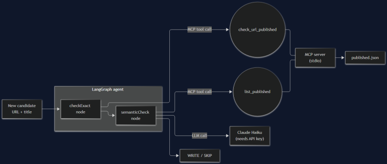
I Built the Agent From Part 1. It's 200 Lines and It Still Broke Once.
Part 2 of the AI agent architecture series: a real MCP server, a real LangGraph graph, and the actual bug — a blog-dedup agent that catches exact-match duplicates fine and faceplants on the semantic case, with a 401 to prove it.
Read more
25 Sep 2026 · 4 min read
ai
CloudWatch Omni: AWS Finally Admits Your Agents Live on Three Clouds
AWS shipped CloudWatch Omni on September 23 — OpenTelemetry-based, natural-language queries, and eval-driven tracing for LangGraph, CrewAI, and Strands out of the box. Here's what it actually replaces and where it still falls short.
Read more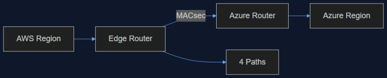
16 Sep 2026 · 4 min read
ai-infrastructure
AWS Just Opened a Private Pipe Straight Into Azure. Here's Why an AI Team Should Care
AWS Interconnect – multicloud with Azure went into preview in August, capped at 1 Gbps and four regions. That's not enough bandwidth for training, but it's exactly enough to fix the multi-vendor inference problem we've been duct-taping for a year.
Read more
Discussion
Comments are reviewed before publication. Your email is kept private.